Actor Temperature
For a history of actor events of length n, we want to calculate an actor’s temperature T, where T is a value form 0 to 1.
When T=0, the actor has not sent any messages that have been classified as toxic.
When T=1, all of the messages sent by the actor have been classified as toxic.
We want to control how much the oldest event impacts the temperature compared to the most recent so we define a discount factor \gamma that is a value from 0 to 1 such that a value of 0 means only the most recent event impacts the temperature and a value of 1 means all events impact the temperature equally.
We define \vec{d} to be the vector of discount coefficients of length n such that:
\begin{aligned}
\vec{d} &= \left[ \gamma^0, \gamma^1, \gamma^2, \dots, \gamma^{n-1} \right] \\
        &= \left[ 1, \gamma, \gamma^2, \dots, \gamma^{n-1} \right] \\
\end{aligned}
We also define \vec{x} to be the vector of actor events where each element is either 0 or 1. A 1 is an event where a message was classified as toxic and a 0 is any other event.
This leaves us with a calculation for T.
T = \frac{
        \vec{d} \cdot \vec{x}
    }
    {
        \sum_{i=1}^n \vec{d}_i
    }
Ok, so this gives us a weighted average. So this is really straight forward, but let’s find a calculation for T when we only know the current temperature and the state of the latest event. This will allow us to update the temperature value without having to store the full events vector.
First, let’s expand this calculation of T and treat the sequence of events as timesteps where t is the current timestep and t-4 is four timesteps in the past.
T_t = \frac{
        x_t + \gamma x_{t-1} + \gamma^2 x_{t-2} + \dots + \gamma^{n-1} x_{t-(n-1)}
    }
    {
        1 + \gamma + \gamma^2 + \dots + \gamma^{n-1}
    }
Let’s also expand the calculation for T_{t+1}.
T_{t+1} = \frac{
        x_{t+1} + \gamma x_{t} + \gamma^2 x_{t-1} + \dots + \gamma^{n-1} x_{t-(n-2)}
    }
    {
        1 + \gamma + \gamma^2 + \dots + \gamma^{n-1}
    }
If we can define T_{t+1} in terms of T_t, x_t, and \gamma then we are finished.
Let’s start by finding an expression that lets us define \gamma x_{t} + \gamma^2 x_{t-1} + \dots + \gamma^{n-1} x_{t-(n-2)} in terms of T_t.
\begin{aligned}
T_t &= \frac{
        x_t + \gamma x_{t-1} + \gamma^2 x_{t-2} + \dots + \gamma^{n-1} x_{t-(n-1)}
    }
    {
        \sum_{i=1}^n \vec{d}_i
    } \\
T_t \sum_{i=1}^n \vec{d}_i &=
    x_t + \gamma x_{t-1} + \gamma^2 x_{t-2} + \dots + \gamma^{n-1} x_{t-(n-1)} \\
\gamma T_t \sum_{i=1}^n \vec{d}_i &=
    \gamma x_t + \gamma^2 x_{t-1} + \gamma^3 x_{t-2} + \dots + \gamma^n x_{t-(n-1)} \\
\left( \gamma T_t \sum_{i=1}^n \vec{d}_i \right) - \gamma^n x_{t-(n-1)} &=
    \gamma x_t + \gamma^2 x_{t-1} + \gamma^3 x_{t-2} + \dots + \gamma^{n-1} x_{t-(n-2)} \\
\end{aligned}
We can now rewrite T_{t+1} as follows:
T_{t+1} = \frac{
        x_{t+1} + \left( \gamma T_t \sum_{i=1}^n \vec{d}_i \right) - \gamma^n x_{t-(n-1)}
    }
    {
        \sum_{i=1}^n \vec{d}_i
    }
This leaves us with a bit of a problem since we can’t know the value of x_{t-(n-1)} unless we store the whole event vector.
The question now is can we get to a “good enough” aproximation of T_{t+1} given T_t, x_t, and \gamma.
We know that x_{t-(n-1)} is either 0 or 1. We also know that \lim_{n\to\infty} \gamma^n = 0 for \gamma < 1. In practice, we won’t be calculating a temperature based on an infinite history but as long as n is sufficiently large \gamma^n will be small. We can then assume that x_{t-(n-1)} represents a toxic message and replace it with 1. This introduces a non-zero error that lowers the temperature value but will be a very small error as long as n is sufficiently large.
With this compromise, we can rewrite T_{t+1} as:
T_{t+1} = \frac{
        x_{t+1} + \left( \gamma T_t \sum_{i=1}^n \vec{d}_i \right) - \gamma^n
    }
    {
        \sum_{i=1}^n \vec{d}_i
    }
If T_t is sufficiently small, we will get a negative temperature which breaks our requiremnets. A small change to the expression allows us to prevent this outcome.
T_{t+1} = \frac{
        x_{t+1} + \max \left( \gamma T_t \sum_{i=1}^n \vec{d}_i \right) - \gamma^n, 0
    }
    {
        \sum_{i=1}^n \vec{d}_i
    }
Granted, we have had to make a compromise to get to this point but the result is we are able to update T without having to know the full history of the actor’s events.
Now let’s double check our requirements.
When x_{t+1} and T_t are both 1, we want T_{t+1} to also be 1.
\begin{aligned}
T_{t+1} &= \frac{
        1 + \max \left( \gamma (1) \sum_{i=1}^n \vec{d}_i \right) - \gamma^n, 0
    }
    {
        \sum_{i=1}^n \vec{d}_i
    } \\
    &= \frac{
        1 + \left( \gamma \left( 1 + \gamma + \gamma^2 + \dots + \gamma^{n-1} \right) \right) - \gamma^n
    }
    {
        1 + \gamma + \gamma^2 + \dots + \gamma^{n-1}
    } \\
    &= \frac{
        1 + \left( \gamma + \gamma^2 + \dots + \gamma^n \right) - \gamma^n
    }
    {
        1 + \gamma + \gamma^2 + \dots + \gamma^{n-1}
    } \\
    &= \frac{
        1 + \left( \gamma + \gamma^2 + \dots + \gamma^{n-1} + \gamma^n \right) - \gamma^n
    }
    {
        1 + \gamma + \gamma^2 + \dots + \gamma^{n-1}
    } \\
    &= \frac{
        1 + \gamma + \gamma^2 + \dots + \gamma^{n-1}
    }
    {
        1 + \gamma + \gamma^2 + \dots + \gamma^{n-1}
    } \\
    &= 1 \\
\end{aligned}
When x_{t+1} and T_t are both 0, we want T_{t+1} to also be 0.
\begin{aligned}
T_{t+1} &= \frac{
        0 + \max \left( \gamma (0) \sum_{i=1}^n \vec{d}_i \right) - \gamma^n, 0
    }
    {
        \sum_{i=1}^n \vec{d}_i
    } \\
    &= \frac{
        0 + \max {-\gamma^n}, 0
    }
    {
        \sum_{i=1}^n \vec{d}_i
    } \\
    &= \frac{
        0 + 0
    }
    {
        \sum_{i=1}^n \vec{d}_i
    } \\
    &= 0 \\
\end{aligned}
Let’s also test that values of 0 and 1 for x_{t+1} have an impact on T that match our intuition of temperature for “real” values of \gamma and n.
Let’s assume n = 30 and \gamma = 0.9.
This results in \sum_{i=1}^n \vec{d}_i = 9.576088417247838 and \gamma^n = 0.04239115827521624
If we start with T_t = 0.5 we end up with the following when the latest event is a toxic message:
\begin{aligned}
T_{t+1} &= \frac{
        1 + \max \left( (0.9) (0.5) (9.576088417247838) \right) - 0.04239115827521624, 0
    }
    {
        9.576088417247838
    } \\
    &= \frac{
        1 + \max 4.309239787761528, 0
    }
    {
        9.576088417247838
    } \\
    &= \frac{
        5.309239787761528
    }
    {
        9.576088417247838
    } \\
    &= 0.5544267718120548 \\
\end{aligned}
And when the letest event is not a toxic message.
\begin{aligned}
T_{t+1} &= \frac{
        0 + \max \left( (0.9) (0.5) (9.576088417247838) \right) - 0.04239115827521624, 0
    }
    {
        9.576088417247838
    } \\
    &= \frac{
        \max 4.309239787761528, 0
    }
    {
        9.576088417247838
    } \\
    &= \frac{
        4.309239787761528
    }
    {
        9.576088417247838
    } \\
    &= 0.45 \\
\end{aligned}
The smaller T_t is, the more impact “warming” has and the hotter T_t is, the more impact “cooling” has. This matches our intuition for temperature.
The following chart illustrates consecutive “warming” and “cooling” events.
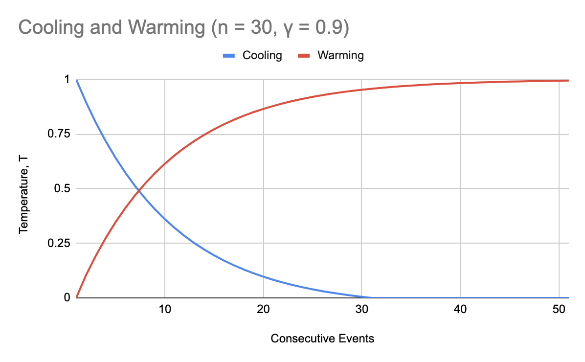
It is worth noting that due to the compromise to prevent negative temperatures and handle the unknown value of x_{t-(n-1)}, the temperature can reach 0 after n consecutive “cooling” events, but the temperature will only ever asymptotically approach 1 as the number of consecutive “warming” events approaches infinity.
TODO: Add coefficients of cooling and heating to enable finer grained control over the relationship between the cooling and heating curves.
NB: The reason I’ve described this in terms of events rather than simply message classifications is that we can define an event as either a message classification or the tick of a clock. This would allow actors to “cool off” by either sending messages that are deemed non-toxic or by simply refraining from sending messages.